2. Methods

Fig. 1 presents the geometry and the pulsatile inflow, which comes from in-vitro experimental 4D flow MRI data based on the same phantom (Garreau et al. 2022). Besides the mesh and boundary conditions, the MR pulse sequence is another input into our simulation, corresponding to the chronogram of the external magnetic field. The MR sequences used in this work are based on a constructor sequence (WIP 4D Flow Siemens). The CFD tetrahedral-based mesh (2mm characteristic size) is seeded with Lagrangian particles (8/cell), which are massless tracers carrying a magnetization vector that evolves with their position and the effective magnetic field they experience. The first step of our solver is to compute the CFD velocity field. This velocity field is then interpolated on the position of particles. Bloch equations are solved for each fluid particle according to the current magnetic events. At particular time instants specified in the sequence, the global magnetization is computed and collected in the so-called k-space, which can be interpreted as the 3D Fourier transform of the image. The synthetic images (SMRI) are then reconstructed from k-space with in-house Python scripts. 

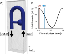
Figure 1 (1) Geometry and MRI field-of-view (FOV). (2) Inflow – Lines indicate time instants for Fig. 2. 

In the present work, two 4D flow MRI sequences are compared, a conventional one and another using partial echo (PE). PE consists in acquiring only a fraction of the k-space, relying on its symmetric properties. Here, the first 25% of the k-space is not acquired for the 2nd sequence. Whereas sequences can be designed so that position- and velocity-encoding occur simultaneously along two directions (here X and Y), there is an inevitable time delay between the velocity and spatial encoding along the last direction (here Z), as the latest has to occur during signal collection around the echo time TE. This delay, called displacement time TD, is known to be related with common misregistration artifacts(Steinman et al. 1997). More than reducing the acquisition time, PE allows to reduce TD. In the present work, the acquisition time has been kept equal for both sequences. TE is reduced from 4.20 to 4.16 ms, but TD decreases from 1.99 to 1.52 ms. Other sequence parameters are equivalent in both simulations. The images of the 2nd simulation are reconstructed according to the zero-filling method (Dyverfeldt et al. 2015).

References

Dyverfeldt P, Bissell M, Barker AJ, Bolger AF, Carlhäll C-J, Ebbers T, Francios CJ, Frydrychowicz A, Geiger J, Giese D, et al. 2015. 4D flow cardiovascular magnetic resonance consensus statement. J Cardiovasc Magn Reson. 17(1):72.
Garreau M, Puiseux T, Toupin S, Giese D, Mendez S, Nicoud F, Moreno R. 2022. Accelerated sequences of 4D flow MRI using GRAPPA and compressed sensing: A comparison against conventional MRI and computational fluid dynamics. Magnetic Resonance in Med.:mrm.29404.
Markl M, Chan FP, Alley MT, Wedding KL, Draney MT, Elkins CJ, Parker DW, Wicker R, Taylor CA, Herfkens RJ, Pelc NJ. 2003. Time-resolved three dimensional phase-contrast MRI. J Magn Reson Imaging. 17(4):499–506.
Puiseux T, Sewonu A, Moreno R, Mendez S, Nicoud F. 2021. Numerical simulation of time-resolved 3D phase-contrast magnetic resonance imaging. Borazjani I, editor. PLoS ONE. 16(3):e0248816.
Steinman DA, Ethier CR, Rutt BK. 1997. Combined analysis of spatial and velocity displacement artifacts in phase contrast measurements of complex flows. J Magn Reson Imaging. 7(2):339– 346.
Keywords: Computational Fluid Dynamics (CFD) ; Hemodynamics ; Magnetic Resonance Imaging (MRI)
Partagez cet article
Share on Facebook
Share on Linkdin
Et si on échangeait ?
Vous êtes praticien ?
Restez informé grâce à notre programme relationnel gratuit pour les professionnels du rayonnement.
Vous voulez devenir partenaire ?
Distribution, R&D, tests cliniques…
Contactez-nous !